
R-squared can be estimated in two main ways:
- Ratio of variance of predictions,
, to that of the response variable, Y.
- A difference between unity and the ratio of variance of residual error to that of the response variable
where
.
For easy communication sake, I’ll respectively refer to (1) and (2) as methods 1 and 2.
These two methods yield identical results and are effective linear model validation measures but only under two conditions:
- In-sample validation: when they are computed with the same data on which the models were fitted; and
- When the model parameters directly estimated from data are used in the R-squared computations.
However, in real world, at least one of the above conditions is almost always violated: It’s recommended practice for scientists to rather validate models on unseen data (i.e. out-of-sample validation). Most model validation in the machine learning era involve computing goodness of fit metrics on unseen data using parameters from competing models. Also, it’s common for scientists to select away from model parameters estimated from data. For instance, in insurance, an actuary can adjust any subset of the estimated model factors for reasons related to marketing, underwriting, regulation or any other he or she deems relevant.
When at least one of the above two conditions is violated, the two R-squared methods, contrary to what have been discussed in statistical textbooks, yield different results, some of which are too consequential to ignore. This paper discusses two of them.
Note 1
The choice of method has two critical consequences on the scientist’s assessment of model fit:
The first is method 1 can produce inflated values and hence overconfidence in the model’s efficacy. To see this, assume:
Assuming further that are the true parameter values, and for simplicity sake, that
and
are independent covariates, then:
Since the denominator of method 1, var(Y), is constant for any given dependent variable, it’s troubling to see that, the numerator, and hence
can be increased by merely selecting parameter estimates that are otherwise different from the true parameters
but larger in absolute magnitude. Particularly, if we predict Y with larger but inaccurate parameters such that
:
then and consequently,
associated with the inaccurate model in (5) exceeds that of (3). Since this is the first time this problem is introduced, I’ll call it the Parameter- inflated R2 Problem.
Another way (1) can yield false conclusions is by the addition of extraneous covariates—explanatory variables that has no relationship with the dependent variable. Suppose one such extraneous variable, z, is added to the model specified in (3):
One can see that, even though the added variable has no statistical relationship with Y, calculated via method 1 will nevertheless increase if
is non-zero. Additionally, if
and the variance of z are high enough, the complexity penalty baked into adjusted
may not be enough to offset the artificial
boost that z provides; when this happens, both
and adjusted
increase. I call this the Extraneous Variable Boost Problem. This problem is broader than the classical over-fitting problem as
may not necessarily have been fitted from data. And also, even though the Extraneous Variable Boost Problem poses a risk to only method 1 (as we’ll see below), none of the two methods is immune to over-fitting problem.
These two problems imply that if the modeler compares different models using method 1, there is a concerning possibility that he or she may choose a model with a higher but a poorer fit. Hence, using method 1 to choose the best model is a dangerous validation approach especially in a modeling aura when the analyst is free to select away from the regression estimates. It also means that in contests where models are judged by method 1
, contestants can cheat by reporting larger parameters and extraneous variables.
Method 2 is free from the two problems discussed above. Because is calculated as the difference between 1 and the ratio of variance of the residual error to that of Y, any inaccuracies or noise in the predictive model augments the subtrahend (i.e. the ratio) and accordingly reduces the difference (i.e.
). In the case of (5), variance of the the residual error will duly increase by
; and in (6), it will increase by
. Before this paper, the two methods had been regarded as equivalent, and the superiority of method 2 had been missed.
Note 2
The second note is that, even though methods 1 and 2 seek to measure the same thing, the two measures have different variances. Hence, using the variance of one method to make inference about the other will yield false conclusions. To show this, consider the following model:
where x1,x2 ~iid Normal(0,1), and ~Normal(0,3) and independent of x1, and x2.
If the above model is simulated 200 times (with each experiment having a sample size of 3000), and the two are computed for each experiment, we observe the following respective distributions:

As can be evidenced from figures 1 and 2, though the two methods yield statistically equal means, the variance of method 2 is twice that of method 1. The reader can infer from the variance formulas below that, when is less (greater) than 0.5, method 1 will have a lower (larger) variance. This disparity in variance, despite the popularity of these two methods, has heretofore not been highlighted. The ramification is that, in making inferences about
, the analyst must use the correct variance for the method he or she chooses. The interested reader should see appendix for the computation of variance of
for both methods.
Conclusion
My two notes are thus these: Use method 2 to compute to avoid the Parameter- inflated R2 and Extraneous Variable Boost Problems; and make sure to use the correct variance for your chosen method in making inference about R2 .
Appendix
Variance of Method 1
The variance of sample calculated by method 1 (i.e.
) can be derived using the delta method as follows:
Where:
In the same vein, the variance of the sample measured by method 2 (i.e.
) can be derived by substituting
with
in the above formulas. One can thus see that the variance of the two measures will be different except for
=0.5 (i.e.
). For a full derivation of (8), see my other paper, G2R2: A True R-Squared Measure for Linear and Non-Linear Models.
References
- Greene, W.H. (2002) Econometric Analysis. 5th Edition, Prentice Hall, Upper Saddle River, 802.
- Kvalseth, T.O. (1985). “A Cautionary Note About R-Squared”. The American Statistician. 39. pp. 279-285.
- Weisstein, Eric W. “Sample Variance Distribution.” From MathWorld–A Wolfram Web Resource, http://mathworld.wolfram.com/SampleVarianceDistribution.html


